lunes, 22 de noviembre de 2010

A proposal on a course on Real-Time Structural Dynamics

 The following is a tree with the key concepts that, although already at reach of any graduated structural engineer, need to be tied together, maybe in a course, in order to achieve a proper scope on how to simulate real-time structural dynamics:
  • Main time integration methods (ODE), their limitations (drawbacks), advantages, motivation, references, illustrations, year, all related to the three disciplines applied physics, maths and applied computing:
      • 1st order
        • Euler
        • Backward Euler
        • Semi-implicit Euler
        • Exponential Euler
      • 2nd order
        • Verlet
        • Velocity Verlet
        • Midpoint Method
        • Heun's
        • Newmark-beta
        • Leapfrog
      • Higher order
        • Runge-Kutta
        • Linear multistep
  • Main constraint/collision (DAE) integration methods, their limitations (drawbacks), advantages, motivation, references, illustrations, year, all related to the three disciplines applied physics, maths and applied computing.
      • Coordinate Partitioning
      • Constraint Orthogonalization
      • Udwadia-Kalaba
  • Main matter/continuum (PDE) integration methods, their limitations (drawbacks), advantages, motivation, references, illustrations, year, all related to the three disciplines applied physics, maths and applied computing.
      • MESH BASED METHODS
        • Finite Element
        • Finite Differences
        • Finite Volume
        • Boundary Element
        • Mass-spring systems
      • MESH FREE METHODS
        • SPH
        • Diffuse Element Method
        • Partition of Unity
        • Moving Least Square
        • Reproducing Kernel Method
A graphical approach to ths subject, not so tied to complex formalisms and formulation, would be a real help to attract more researchers into this fascinating discipline.
It also would reinforce the interest on the very differential equations, as these are a very abstract concept explained and taught on a very abstract basis. This makes them first candidate to be either forgotten or banned into the minds of students.

I will try to develop these subjects with more care in future issues...

Se vidimo!

martes, 26 de octubre de 2010

Physics Engines Benchmarking

The target was to devise in some manner the way different computational physics simulation models/engines/environments performed against a canonical one.

For such purpose, I have reviewed the paper "Beam Benchmark Problems For Validation Of Flexible Multibody Dynamic Codes" by A.L. Schwab and J.P. Meijgaard.
The following is an outline of the proposed in this paper:

  • 1.- Introduction
    • The paper presents some basic problems for which analytic solution is known
  • 2.- Beam benchmark problems
    • Tests to be performed
      • Static analyses in small displacements for the validation of the correct formulation of elastic forces
      • Static analyses for large displacements and rotations, on straight and curved beams
      • Buckling tests in normal, lateral and torsional directions to check the way geometric stiffness due to prestress is taken into account
      • Eigenfrequency analyses for the validation of the combination of elastic forces and distributed inertia forces
      • Mesh refinement tests for all the above to prove convergence of the results
    • Underlying model: Timoshenko beam with large displacements and large rotations
      • Finite Element Method Beam Element
      • Shear flexible based on the elastic line concept
      • Slender beam, cross section doubly symmetric
      • Large rotation and displacements, but small deformations
      • Isotropic and linearly elastic
      • BEAM model: standard strain-displacement relations
      • BEAMNL model: additional quadratic terms included in the strain-displacement for better performance in the pre-stress cases
Interestingly enough, the analytical solution is provided for each of the tests, and the proposed model is simple enough so as not having too much trouble in introducing it in a few characteristic ready made softwares currently available.

The implementation of such a benchmark over some of the most popular engines revised lately would surely make a nice contribution.

jueves, 14 de octubre de 2010

Integration Overview

In order to get some scope I have prepared a new diagram where the different integration fields of any multibody physics engine can be fit.
Normally we have to integrate time, via ODEs, for which any of the available schemes can be chosen, but then also the Differential Algebraic Equations for constraints (related to collisions) and the Partial Differential Equations related to the continuum have to be solved.

Of course, not every engine implements the continuum part (limiting to rigid solid) and some matter integration schemes already consider the very collisions so the constraint integration is explicitly sorted...

The associated disciplines where each concept fits are represented by the horizontal blocks.


miércoles, 22 de septiembre de 2010

Discipline Overview

Holidays are over already. I am now living in Slovenia, Ljubljana, and developing the thesis in the Faculty of Architecture (lovely place, by the way...).

Last June I presented my Thesis Proposal to the jury of the Computational and Applied Physics Department in the UPC and...it was accepted!!

After the long pause I have had to prepare an overview of all the studied subjects, just to get some scope on what is coming and where we are now. The following diagrams give some idea on how it is:


And with a bit more of detail:

These diagrams derive from the need of disentangling disciplines that more often than seldom get mixed in the literature and make it fairly hard to follow.
The literature I am talking about is that of the computational simulation of physics, where numerical methods meet with very different origins.

martes, 27 de julio de 2010

SUSTAINABLE DYNAMIC STRUCTURES WITH CANE

The last month I have been quite busy helping out raise the structure above.
It is located near Idanha Velha, in the premises for the International Boom Festival in Portugal.

It is one of the most clear examples of dynamic structures, where ordinary laws of statics don't apply, and one of my first fields of intense research.

The aim is to reach a comprehensive computational model that allows the designer (Jonathan Cory Wright - www.canyaviva.com) to experiment with his designs prior to having to actually raise his buildings!

martes, 20 de abril de 2010

An Overview on Constraint Enforced Formulations of Variational Dynamics

A couple of weeks ago a very interesting paper entered my hard drive: Review of classical approaches for constraint enforcement in multibody systems.
It is a fairly clarifying overview on solid grounds of certain methodologies to solve multibody systems dynamics.
These methodologies differ from the ones I have encountered in the spreaded dynamics engines in their apparently more robust and simple formulation.
Here is a synthesis of this paper:

Multibody systems present two distinguishable features:
  1. Bodies undergo finite relative rotations, which introduce nonlinearities
  2. Bodies are connected by mechanical joints that impose restrictions, which mean a set of governing equations that combine differential and algebraic equations (ODEs and DAEs, respectively).
Lagrange's equation of the first kind has the following aspect:
Where
  • M=M(q,t) is the mass matrix
  • q is the generalized coordinates vector
  • B is the constraint matrix
  • λ is the array of Lagrange multipliers
  • F is the dynamic externally applied forces
If all the constraints are holonomic (velocity independent), B is called the Jacobian matrix, and the generalized coordinates, q, are linked by m algebraic constraints.
Lagrange's equations of the first kind form a set of (m+n) Differential Algebraic Equations.
The approach of the following methods is to use algebraic procedures in order to eliminate Lagrange's multipliers and then obtain a set of ODEs.
  • Maggi's formulation: implies the creation of a vector containing the so called kinematic parameters, generalized speeds or independent quasi-velocities by the analyst in order to obtain a Γ matrix. This matrix spans the null space of the constraint matrix and allows for the elimination of the Lagrange multipliers.
  • Index-1 formulation: requires that initial condition of the problem be subjected to the constraint conditions. Then, it is possible to obtain a system of 2nd order ODEs that is solvable by rearranging the previous equation, extracting the Lagrange multipliers and hence obtaining:
  • Null space formulation: this method solves the system of second order ODEs by premultiplying the first part of the equation by the transposed null space matrix thus eliminating the Lagrange multipliers.
  • Udwadia-Kalaba formulation: this method represents a more compact and general form of solving the DAEs by means of the Moore-Penrose generalized inverse. It is based on Gauss' Principle of Minimum Constraint, which establishes that the explicit equations of motion be expressed as the solution of a quadratic minimization problem subjected to constraints, but at the acceleration level.

All these formulations transform the (2n+m) first order DAEs into ODEs by eliminating Lagrange multipliers.
Maggi's formulation yields (2n-m) first order ODEs.
Index-1, null space and Udwadia-Kalaba form sets of (n) second order ODEs which could be alternatively recast into (2n) first order ODEs for the n generalized coordinates and the n generalized velocities.
The main advantage of these methodologies is not so much the reduction in the number of equations but rather in the change from DAEs to ODEs.
There is a warning on the constraint drift phenomenon, for which these method will be more affected (not so much in Maggi's formulation), and that would require constraint stabilization techniques.
My conclusion is that it seems the way to go, not only for the claims of more stable and quick numerical techniques available to get them working, but also for an apparently more clear approach in the theoretical field.
Particularly, I have done some research into the Udwadia-Kalaba formulation, and definitively is a very promising one.

jueves, 15 de abril de 2010

ODE DYNAMICS ENGINE QUICK OVERVIEW

After seeing my own simulator running there is a whole lot of things that I wish it had.
All this stuff is more or less complicated to achieve, but from my previous research I have found some Open Source engines from which I can learn a lot.

The best documented one so far is ODE (www.ode.org), and also the one I intend to merge with Blender.
So, I present a very quick and thorough overview on how this works, in order to have some scope.

The first thing to disentangle is how it gets working. For that, just looking at the user's manual one gets the following algorithm:

1.-Create a Dynamics world
  • This basically means to make an instance of the dxWorld struct.
2.-Create the bodies
  • Attach the bodies to the world (this means adding data to the dxBody* array of the dynamics world).
  • Set their properties (position and orientation of point of reference, its linear and angular velocities, the mass of the bodies and some other stuff of the like).
3.-Create the joints
  • Attach the joints to the world (by adding data to the dxJoints* array of the dynamics world)
  • Set their properties (depending of the selected type of joint, one has to provide different details).
4.-Manage collisions
  • Create a new collision world (just by making an instance to the dxSpace struct).
  • Create a joint group where collisions will be stored temporarily for every frame step.
5.-Loop
  • Apply forces to bodies.
  • Adjust joint parameters.
  • Call collision detection.
  • Create a contact joint for every detected collision point and add it to the collision joint group.
  • Take a simulation step.
  • Clear the collision joint group.
6.-Destroy the dynamics and the collision worlds (wow, that sounds evil...hehehe).

All of this seems fairly easy to do but then one has to get to know where and how things have been implemented. This is when things become a bit harder.
I am sure the file structure and the class definitions make perfect sense for the programmers of this engine.
Fortunately, they have been careful enough so as to comment everything in an understandable way, for which I feel deeply grateful.
After some digging, I have managed to restructure the ode/src folder into the following topics:
  • Accessories
    • Memory management
    • Math
    • Matrix handling
    • External applications
  • Collision
  • Core
  • Joints
  • Primitives
  • Solver
Which means one can tackle the engine in an ordered manner and find things when needed.

From a theoretical point of view, this engine presents the following features:
  • A Lagrange multiplier velocity based model from Trinkle and Stewart
  • A friction model from Baraff
  • A Danzig LCP solver

martes, 13 de abril de 2010

First Ogre+Verlet+Gauss-Seidel simulation

Once the Ogre3D engine is ready to draw what we numerically compute, it was about time to start having some fun.

I found this excellent article from Thomas Jakobsen: http://www.gotoandplay.it/_articles/2005/08/advCharPhysics.php where a very neat and simple engine is implemented (thanks Mr. Jakobsen).

It is very well explained so adapting it to my little lab was not very hard.
Here I proudly present my very first simulation!


I am perfectly conscious that it lacks of a lot of things...namely collision detection, a proper stable, precise integrator, an optimized implementation...and a long etcetera...but it's just a baby!

Here is a zip file with the code (an extension from what I presented in the last post):


http://www.mnbvlabs.com/Thesis/VerletRelaxation.zip

domingo, 11 de abril de 2010

Setting Ogre3D as Graphic Environment

The last days I have been working on getting a Graphics Environment for my Toy Physics Engine.
Last December and January I had already fiddled around with excellent engines Ogre (www.ogre3d.org) and Bullet (http://bulletphysics.org/wordpress/), trying to put them to work together.I have a post from february where some simulations on youtube can be seen and some preliminary introductions are made.

However, now I am starting to understand things, and whenever I have the drive to test them always encounter the problem on how visualize them.

So, I came across with Blender (www.blender.org), another fantastic tool, and got surprised to find their Google Summer of Code mentorship for 2010 (http://wiki.blender.org/index.php/Dev:Ref/GSoC/2010/Info).
I have applied for it. Deadline was 9th April, which meant preparing everything in a hurry and some embarrasing trouble with their wiki page (I have already apologised in their bf-commiters mailing list...ooops).
Here is my proposal for such an important event: (http://wiki.blender.org/index.php/User:Ndujar).
Hopefully they find it interesting and contact me to complete it!

In the meantime, I have prepared a short and basic Ogre framework to begin doing some tests.
It is composed of a few files and classes integrating Ogre.

I generated it basically copying, cutting and pasting from the very good tutorials available at the Ogre web page (http://www.ogre3d.org/wiki/index.php/Ogre_Tutorials).

It goes as follows:

The first step is to intall and cofigure Ogre in your computer. This is the best tutorial I found: http://ubuntuforums.org/archive/index.php/t-1148570.html.

Then, using whatever IDE of your taste (I am on EasyEclipse), just get the following files to compile.

The core of the application is the BaseApp object, from which I will later extend further as needed. It is basically in charge of doing everything Ogre requires to be done to put things up in a rendering window.
BaseApp.h:

BaseApp.cpp:


The BaseFrameListener is another very important piece of code that allows one to control the rendering flow.
In order to manage whatever happens on every rendering step, Ogre provides the FrameListener object.
With the installed package comes an ExampleFrameListener.h file, which overrides the basic Ogre FrameListener and allows for a fairly good control over the inputting devices such as keyboard and mouse.I have slightly customised it for my purposes.
It has been a bit tricky however, and has made my computer crash a few times.
Anyway, here it is, domesticated at last!


BaseFrameListener.h:


Once the beast is under control, the rest is a piece of cake...hehehe... 
You can make as many instances of a FrameListener as you need in an Ogre application.
I have chosen to create a separate framelistener for managing whatever goes under the physics, to keep things up neat and tidy.
It is the PhysicsFrameListener class:

PhysicsFrameListener.h:


The elementary brick on which everything else will be constructed is likely to be called PhysicsEntity.
So I have defined my PhysicsEntity Class.
In this code is still at its very bones, just presenting a couple of functions to make things visible.
Hopefully in the near future some more flesh will get added on it!

PhysicsEntity.h:

PhysicsEntity.cpp:


Last, but not least, is the main.cpp file, where everything gets blended:

main.cpp:


And this is it. Now...Let's get busy!

miércoles, 31 de marzo de 2010

CODE NAME: Brachistochrona

Today I'm going to reveal a classified archive. Or so it seems...

Physicians have been keeping this knowledge from us simple mortals for centuries...hehehe...
While trying to understand the essentials on variational mechanics, I have come into this article: http://jazz.openfun.org/wiki/Brachistochrone.
The problem of the brachistochrone dates back to Newton (17th century) and appears mentioned frequently as one of the problems that can be solved be means of this refined technique.

In fact, this problem appears to be the actual trigger for the modern physics (or better stated, its solution), and reveals a completely counterintuitive phenomenon:

The quickest path is not the straight line

Amazingly, the solution for a bead on a wire going in the least time from point A to point B:


Is the cycloid represented in the picture.

As standard human, one always tends to think that the shortest path would be the quickest one. It is wrong.
Analogously, when it comes to minimize the action (see previous posts on the subject), it is very hard to imagine that the stationary points would not come at flattening the curve for the action.
This is what makes so hard to understand the variational principles that rule over Lagrangian, Eulerian and Hamiltonian mechanics.

If one only had been told...

I have made a spreadsheet with openoffice (www.openoffice.org) where this can be numerically perceived also.

The spreadsheet is here.

I have made it with the help of a paper by Jozef Hanc: The original Euler's calculus-of-variations method: Key to Lagrangian mechanics for beginners.
I found it extremely appropriate for my case, and also absolutely clarifying. Thanks mr Hanc

domingo, 28 de marzo de 2010

Ilustrating Lagrangian Variables

In the last post we had a tentative on Variational Mechanics which resulted very stimulating.

In order settle ideas down, I have left the subject cooling in the fridge and I have fiddled around with the Lego Mindstorms(c) robot we have at the RGEX research group, trying to make a positioning system that is accurate enough for our purposes.
Surely Jaume (my thesis director) will be very happy to hear about it.
I know this is not the exact place for it, but it's my blog and I do what I want to...hehehe...anyway, whoever wants to see what we do there, it is available at: www.rgex.blogspot.com.

And now, back to work:

The intention of this post it to illustrate some relationships that exist in Mechanics and that are repeated ad-vomitum in every reference one finds on Variational Mechanics.
The main problem I have encountered is that explanations mix numerical methods with physical concepts, and more often that seldom everything is written in the cryptic language of mathematicians. Of course, in complete absence of figures or anything of the like.

So, here we go...
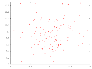
With the help of some coding in C++ and QtOctave (https://forja.rediris.es/projects/csl-qtoctave/), I have made some graphics for the simulation of a moving particle.
I have used the same deductive principle I have seen in the papers, which is not intuitive at all. Hopefully some drawings will make it more clear.

A moving particle

Instead of trying to obtain the formula in a straightforward manner, the Least Action Principle suggest one to imagine an arbitrary particle that changes its position from one place to another. So, that's exactly what I have done.
The code iterates some 100 times and assigns random values to the new position of our particle. Really simple stuff.


The red dots represent all 100 different positions the particle goes when random increments in x and y are applied.
The initial point is at (10,10), and all the following are dQ further (dQ is divided in X and Y components, of course). dQ gets a random value for each iteration.
Once we have the new positions, it is straightforward to apply physics concepts to get the values of Velocity, Acceleration, Kinetic Energy and Potential Energy that have to be applied to get the particle there:

V=dQ/dt
A=dV/dt
Ep=m*A*dQ
Ec=1/2(m*|V|²)

With a dt value of 0.1 and a mass m of 5, it is also a piece of cake to obtain a table with the respective values.

Work and energy

The magnitudes Work and Energy are directly related to the Ep and Ec values.
From a physical point of view, there are some very interesting things that can be observed when putting their values against the |dQ| values:

Distance |dQ| vs kynetic energy Ec
Distance |dQ| vs potential energy Ep

From the same experiment, the random values of distance show a correlation of two types with the respective energies: 
  • Kynetic energy is linearly related to the distance covered by the particle. Its values depend solely on the module of the velocity parameter, which itself is linearly dependent on the distance.
  • Potential energy shows a more quadratic behaviour, provided its acceleration component is multiplied by the covered distance.
It is also interesting to have a look at the graph Ec vs Ep, where also the quadratic behaviour is observed:
Kynetic energy Ec vs Potential energy Ep

Interestingly enough, both (|dQ| vs Ep) and (Ec vs Ep) are exactly the same shape, but for the scale of the X axis, which is of course linearly related.

The basic variational principle

The following step once these observations are made, is that of nesting our little freely moving particle loop into another broader loop, and accumulate the values of the position to form a trajectory.

Provided the inner loop generates a bunch of 100 probable future positions, one tempting criterion would be to choose that of minimum value for the total calculated energy...
The random accumulated trajectory of the particle

Just to verify that by adding the minimum energy substeps we still get a random trajectory.
Obviously, no constraints have been applied, and the particle represents a "Markov process".
What the basic variational principle teachs us is that, given certain constraints, the trajectory of the particle would have been that of minimum energy.
In our code for each time step the chosen subpath has been that of minimum energy.
Nonetheless, for the global trajectory, i.e. after a series of timesteps, a more holistic approach has to be taken in order to obtain the actual "natural" path.
That is the ODEs approach, and we'll talk about it in further episodes...

The following is the C++ code employed to obtain the tables. These have been plotted with QTOctave, an opensource version of MathLab.
Please note that it is the version which provides the complete path. The inner loop provides the random new positions and the outer loops concatenates one position after another, selecting each time that with the minimum energy.

main.cpp:

sábado, 20 de marzo de 2010

ACTION!

One more week spent on Lagrangian Dynamics...and more results!

Well, the main point about Lagrange and his ubiqutous formulae (that following level of abstraction I talked about in the last post), passes through the concept of ACTION.

Inexplicably, when learning physics at the Secondary or even at the Graduate studies, everything seems to finish when we get to the three laws of Newton.
That's the highest point one ever gets...and then we reach the concept of energy by integrating forces along paths.

But there is still one step further (or maybe more, now that the world seems to be round instead of flat, one never knows...).

The notion of action is that of the integral of the energy along time. Easy, isn't it? Its units are energy·time (Joule-second in SI).
Ok then. The problem, I guess, is that in order to be able to do something useful with it, one has to go also one step further in the mathematical notion of function: that of Functional.

And perhaps here is where our poor brains become at risk of melting...or maybe not, because a functional is just a function where the variable is...a function.

So, we are supposed to understand and memorize the linearity property of the integrals, and not the idea of functional? Come on...

Anyway, let's forgive our poor teachers of calculus and physics, who did their best I am sure, and get to work...

The discipline in charge to explain functionals is Variational Calculus, a fairly complex matter. When applied to physics, it happens to produce the Variational Principle of Physics, which is on where all Lagrangian, Jacobian, Hamiltonian and Eulerian dynamics rest.

So , in order to properly grasp the ideas of Lagrangian Dynamics, we better start with a little revision. The best one I found is from Mr. Claude Lacoursière's thesis "Ghost and machines: Regularized Variational Method for Interactive Simulation Multibodyes with dry friction" , combined with the following extremely clear explanation of the concept of action (http://wapedia.mobi/en/Action_(physics)):

1.-Work and Energy:

When a force is applied over a mass along a trajectory kinetic energy is dissipated. Integrating the formula, we can obtain its value as:

                                        T(x')=(m·||x'||²)/2

where x' (aka velocity) is the derivative of the position, m is the mass of the particle and T(x') is the total kinetic energy.

For the cases when the force assumes values tangent to the energy function, then another form of energy appears: this is potential energy. 
This special form of energy has the special property of being independent of the trajectory.


And this form of energy must also be considered into our energy equation if we want to account for everything.
This leaves our equation for the energy of the system the following way: 

                                                  E=T(x')+V(x) 

Being T(x') the kinetic energy described above and V(x) the potential energy.


2.-Basic Variational principle:

Once we have our Energy Equation, we are able to define the Action S for that Energy.
This would be, as explained above, the integral of this equation over time.


Here, t1 and t2 are the initial and final time positions, and L(x,x') is our LAGRANGIAN, which is exactly our Energy Equation, but with another name.

The funny thing about this integral is that it solves nothing by itself. There is a lot of possible solutions for our trajectory, all of them valid in mathematical terms, but only one of them is good for us.


The D'Alembert principle states that, "for a physical trajectory and infinitesimal displacements thereof at each point in time, and compatible with all imposed constraints, the work done by the virtual displacements along the trajectory vanishes when the motion is not bounded, and non-positive otherwise".
In plain English: the path followed is going to be that for which the action is minimized (or more strictly, for which the action is stationary, i.e. there is a minimum point).


To express the constraints mentioned by monsieur D'Alembert, all we need is to apply Euler-Lagrange equation:

                                             ∂L/∂xi - d/dt ( ∂L/∂xi' ) = 0

And then use the mathematical technique of the Lagrangian Multipliers (which I will not explain here), in order to simplify our Action Integral into something we can operate with, i.e. a second order differential equation.

And this is it. The basis, the cornerstone of Lagrangian Dynamics, demystified.
Once these concepts are comprehended, it is relatively easy to toddle around all the rest of this vast world...now at least we have legs!


domingo, 14 de marzo de 2010

LAGRANGIAN DYNAMICS

These days I've been researching on Lagrangian Dynamics.

Finally, some light has been shed through the thick mesh of formulae, technical and mathematical verbiage, and an atom of understanding has entered into my banged head.

The paper that has finally put everything together is this:

http://box2d.googlecode.com/files/GDC2009_ErinCatto.zip

But before, I have had to go through an odissey of other papers to understand why they call it Lagrangian Dynamics, and Lagrangian by extension, to everything related to dynamics in the latest physics simulation R+D world.

The thing is as follows, explained in plane English for plane human beings (like myself, ahem...):

Classical Newtonian mechanics have some limitations when it comes to computing the equations of motion.
We want to iteratively solve a set of Ordinary Differential Equations (ODE) for acceleration, velocity and position if we want to know where our physical elements will be.
But it happened that mysteriously, when computing them, the total energy of the system got affected, because dissipative forces like damping, friction, etc... had to be also implemented, at that is a daunting task...

And there is where Lagrange comes into play: he theorized that we can make use of a further abstraction of our system and embed it into another, a bit broader conceptually, where all these forces would not be so determinant and we still could retrieve our results for position, by applying energetic conservation concepts.
Of course this abstraction comes at the price of having to understand a lot of many other things, not simple either (one funny thing about all this is that the only examples I have been able to find are that of a pendulum, a spring tied to a mass and a bead on a wire...If you didn't get it at the beginning, you'll never do...until you get it. Then these are so obvious you can't think of another!)

Anyway, the main point on Lagrangian approach to dynamics is that we can (and we normally do) find a set of equations that constraint the movement so the energy of the particles individually remains untouched.
These constraints materialize in the form of Jacobian Matrices or Lagrange Multipliers applied to each particle, rigid body or mass in a mass-spring system into our simulation (this is much deeper explained in the paper).

Fortunatelly also, all the above can be applied to Finite Element Method meshes. All we have to consider is that, in Lagrangian dynamical FEM, instead of having only one term for the stiffness matrix as usual:

                     [F]=[K]·[u]

a few more matrices that represent the dynamic terms appear:

                [M][u''] + [C][u'] + [K][u] = [F]


And this is it regarding brand new concepts. It is as far as I can go by now.

In the way I have encountered many intensely related diverse topics, which should be explained in following posts. Some of them are:
  • Linear Complementary Problem Solvers
  • Principle of Virtual Work
  • Differential Equations
  • Smoothed Particle Hydrodynamics (SPH)
  • Kynematics
But for now I will leave this introduction as it is

miércoles, 10 de marzo de 2010

Stiffness Method and SBRA

Eventually I have managed to implement the full code for a simple Direct Stiffness calculator.
The previous post has been conveniently modified to reflect this.

The results have been fairly discouraging for my intemptions to use it as a basis for the SBRA: initial research led me to the wrong idea that the most computationally intensive part was that of assembly of the stiffness matrix, but my own experiments have proven the opposite.

The code provided, on a 1.66 GHz processor (the computer is actually dual core, but no parallelization was used), with 2GB RAM, takes 46 seconds only in the solving part. The modelled structure is 1000 nodes and 1800 elements large.

According to the paper, about 10⁷ iterations are needed over the solver to get a proper reliability assessment. Hence, grosso modo, applying SBRA to this structure on this computer would take 46*10⁷ seconds, some 14.5 long years.

It is likely that, for smaller structures and using parallelization, times become significantly smaller.

Nonetheless, the point I wanted to make here is that of the solving step being the most computationally intensive, instead of the presumed assembly step.

viernes, 5 de marzo de 2010

DSF Implementation

Well...the following is the C++ code to achieve the initial stages of the DSF (e.g. member formation, globalization, merging and linear solving):
main.cpp:

Element.h:
Element.cpp:
Node.h:
Node.cpp:
 
Stiffness.h:
 
Stiffness.cpp:


I have used the GSL library for everything related to maths (http://www.gnu.org/software/gsl/).
This will make my life a lot easier once I manage to master it...Is fairly well documented, so it won't take long (I hope).
Please note that to make the timer work, under Ubuntu 9.10, I've had to activate the -lrt tag in the linker.

miércoles, 3 de marzo de 2010

Direct Stiffness Method

Well...as promised, these past days I've been researching on the possiblity of efficiently use the SBRA through the application of MonteCarlo methods.

I have been successful in my research and I have found this very interesting course:

http://www.colorado.edu/engineering/cas/courses.d/IFEM.d/

It is extremely complete!!

I have used it to refresh my rusted matrix knowledge from my university years, and so far I have managed to implement a very simple program - though effective for my purposes - that will allow me to benchmark the most time-consuming tasks in classical analysis.

This is a very brief resume of the algorithm from the course outlined above:

DIRECT STIFFNESS METHOD STEPS
  • Breakdown
    • Disconnection
    • Localization
    • Member Formation
  • Assembly 
    • Globalization
    • Merge
    • Application of boundary conditions
  • Solution
  • Recovery of derived quantities
The code provided in the course is for Mathematica®, so all I have to do is translate it to C++.

I will provide the lines of code in the following posts.

jueves, 25 de febrero de 2010

Simulation Based Reliability Assesment (SBRA)

This is the resume of the papers:
Both developed under supervision of Pavel Marek (see previous post about structural engineering conception).

The first one is very interesting since allows comparison between the actual "State of the Art" (i.e. Limit State approach to design), and the proposed explicitly probabilistic approach.
It describes a step-by-step process of analysis and design comparing both methods:
  • Loading and load combination
    • LRFD/Limit States
      • Each load is expressed by nominal value and its load factor
      • Load combinations are determined according to rules established in the Codes
    • SBRA
      • Each load is expressed by a load duration curve and its corresponding histogram
      • Load combination employs Monte Carlo sampling over some 10 million iterations of the analysis
  • Resistance and reference values
    • LRFD/Limit States
      • Resistances are combined with different resistance factors associated with failure mechanisms (yield stress, compression, flexure, shear,...) also provided by regulations
      • Design capacity=Nominal capacity x provided failure factor
    • SBRA
      • Reference value corresponds to the onset of the stress/deformation curve of the material when reaching yielding, or to a tolerable deformation
      • An histogram of yield stresses is used to feed each analysis iteration altogether with the histograms for the loads mentioned before
  • Frame analysis
    • LRFD/Limit States
      • One single iteration is made
      • Direct 2nd order analysis can be used, in order to check stabilities, but the most common approach is to do a 1st order analysis and then modificate it
    • SBRA
      • Analysis is repeated 10 million times using each time the values for loads and resistances extracted from the corresponding histograms. In these histograms, the more probable a load or resistance value, the more often will be used. An histogram is also called Probability Density Function in Monte Carlo literature.
      • Initial imperfections are explicitly taken into account
      • There is no need to check individual stability of columns (2nd order)
      • Resistance is related to the onset of yielding
  • Safety assessment
    • LRDF/Limit States
      • Once analysis is computed, for each element we check that the relationship Demand/Capacity is smaller than one
    • SBRA
      • Probability of failure Pf is compared against target probability Pd provided by the codes
      • P[(RV-LE)<0]=Pf
        • RV=yielding stress
        • LE=calculated stress
The proposal is very interesting in terms of  providing a controlled design and an explicit probabilistic model of the structure.

Nevertheless, anyone would encounter the main drawback in the need for iterating 10 million times the whole structure, specially when it comes to real-time Lagrangian dynamics, as we are aimed to.
The steps for modelling the forces and displacements remain the same, it is, the traditional stiffness matrix.
Further research shows that the main time-consuming step into the stiffness matrix procedure (also applicable to FEM) is that of the assembly of the stiffness matrix (60-80%).
This means that, once a configuration is achieved and assembled, solving the matrix with different load cases should be relatively quick. Which is a relief if we want to implement SBRA.
Nevertheless, I still feel like I should pay deeper attention to this speed subject, and obtain my own benchmarking.