WHAT DOES SHAPE FUNCTION MEAN IN FINITE ELEMENT FORMULATION?

Finite Element Analysis is a mathematical tool very extended among engineers. However, after more than a year researching on the topic of computer simulation, where FEA plays such an important role, I haven't yet found a satisfactory explanation on how they really really work...
Hopefully by means of this post I get to clarify some of the topics, trying to remove excessive algebraic and mathematical verbosity that is so annoyingly present everywhere.

The main background of FEM is that of structural engineering in the 60s. Engineers are very practical people, so initially they devised a system which allowed them to set algebraic equations where the relations between different points or "nodes" of their structures could be set.
These algebraic relations were further proven to be of many different types, not only structural, so also thermal relations could be formulated and many others: all one needed to analyze was a proper discretizacion of the space in the form of a mesh with nodes to relate to each other.

For our particular case of  structural engineering (the one that matters for my PhD thesis),  I have tried to illustrate the procedure in its three main steps, so the main ideas come up in a graphic taste:

STEP 1: Discretization
In this basic yet classic example, I have chosen to divide my sample structure in only 5 elements where nodes are clearly identifiable in the meetings between beams. There are four nodes.

Degrees of Freedom

Each node will have 6DOF (Degrees Of Freedom): three for linear displacement on each axis (X,Y,Z) and three for rotational around each axis (X,Y,Z), because we are working on 3D. Many examples available provide the more "simple" 2D situation, but in my opinion this only complicates things further.

A sample structure (mesh) and its topology table

Once the nodes are located and there is a network of how they relate to each other, we can consider we have a mesh. In our example, the correlation is depicted in the table: The elements serve to "link" nodes to each other. The table establishes a "topology" for the nodes.

STEP 2: Element characterization and shape functions
In this step is where FEM formulation and literature get really really awkward and nasty. In fact, this is the core of everything and where FEM differenciates from other ways of solving PDEs.

Different types of Finite Elements

In reality, and despite its mathematical complexity (also unneccesary to be explained so much in detail in my opinion), what we are looking for is a way of characterizing the material properties of the element. For such purpose, the method requires that the behavior of those links among nodes obeys some formula. This formula is the actual Shape Function. In fact, the shape function can be any mathematical formula that helps us to interpolate what happens wherever there are no points to define the mesh. This "ghost" entity that appears between nodes is in fact the Finite Element. In practical terms, as engineers we are more interested in the implementation of the FEM, not so much on its formulation, so what is important to understand is that for different shape functions we obtain different element matrices.

2DOF Beam element matrix

3DOF Beam Element matrix

3DOF Timoshenko Beam element matrix

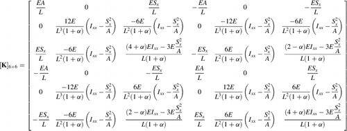
 6DOF Timoshenko Beam element matrix

Depending on the chosen formulation we have different degrees of interpolation and hence presumably higher or lower degrees of precision. Also depending on the chosen formulation we might have different ways of locating and relating our nodes to each other.

For our example we can choose any of the formulations provided in literature (above are the most common used in structural engineering). It is important to note the internal structure of these element matrices, which are symmetrical and clearly divided into parts each corresponding to the nodes that reside on the element's boundaries (2 nodes in the case of a beam - 4 quadrants in the matrix).

STEP 3: Matrix assembly and solution

Because the relations between nodes need to be accomplished all at the same time, we have to set all the equations in such a manner that they compose an algebraic system of equations. The matrix equation we want to solve (at least in statics) is as follows: 

[F]= [Kg]·[u]

Where [F] is the vector of applied external forces, [Kg] is the system's global stiffness matrix and [u] is the vector of displacements resulting from the application of the forces. The size of [Kg], [F] and [u] is that of the number of DOFs times the number of nodes, being [Kg] squared and [F] and [u] unidimensional.

In order to generate the Force vector, all we need to do is collect the applied forces (linear and moment forces) and sort them according to the index of the node they are applied to.

For the global stiffness matrix, it is necessary a bit more laborious procedure by means of which we iterate throughout each element's particular stiffness matrix. Out of each one of those, we get only the part that corresponds to the position of the node we are storing in the matrix, and add it to the possible concurrent data that comes from other elements. Warning: before entering in the global stiffness matrix, we must convert local coordinates to global coordinates!

To get the displacement vector, it is needed to first enforce the constraints and then solve the resulting algebraic system of equations. To do this there are two classical approaches: Penalty Method and Lagrange Multipliers method, but we wont enter into this here...

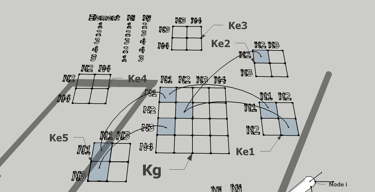
Global Matrix Assembly

Afterwards, all we need to do is use any available algebraic equation solver (LU decomposition is one of the most extended), and obtain the solution of the system.

Impulses, FEM and Verlet

After some time struggling with formulations of many diverse categories, I have eventually managed to implement a computer program where the scheme explained in the november entry ( A proposal on a course on Real-Time Structural Dynamics) becomes clear and useful. The main point here is to explain how, by organizing the numerical methods according to what they really discretize, it is possible to grasp and understand such an entangled area of knowledge. One of the main difficulties that I am encountering through this research period is not just that of the thick mathematical language employed but mainly that of mixed concepts when authors come to explain each of the endless methods available in literature. The following is an step by step procedure where time, constraints and material properties are respectively integrated by means of Verlet, Impulse formulation and Finite Elements numerical methods. The software framework for development and visualization is that presented in April 2010 (one year already uuf!): First Ogre+Verlet+Gauss-Seidel simulation. On top of it I have made the necessary modifications and also the adaptation from Linux to Windows so it is easier to make further comparisons with commercial codes. The first that is needed is a set of nodes with their coordinates and their masses, along with the list of constraints that topologically relate one to another and to the environment:

Time integration: Verlet ODE integration method is known to have certain stability but not a big deal of accuracy. However, is fairly easy to implement. An exhaustive explanation on how it works can be found here: http://en.wikipedia.org/wiki/Verlet_integration. In our implementation, it is divided into functions: AccumulateAccelerations and Verlet.
In AccumulateAccelerations we iterate through each mass and add up earthquake readings from a file (per millisecond), gravity acceleration (980 cm/s2), and the internal forces caused by deformation divided by the weight of the mass.
The Verlet procedure, simply updates the position of each particle according to the formula: 

x(t)=x(t-1) + v(t)·dt + a(t)·dt^2

Constraint integration: The only constraints included in the current implementation are those of the distance between two particles. By means of the concept of impulse, once two particles move close or apart by the effect of the accelerations, a corrective force is applied on each one of them. This force is applied in a very short lapse of time, hence can be regarded as an impulse. A more detailed explanation can be found in the work by Jan Bender (www.impulse-based.de). The algebraic system of equations that arises so as to satisfy all of the constraints simultaneously is solved by means of a Gauss-Seidel iterations.

Matter integration: For the consideration of matter properties the program uses the Finite Element Method. A quadratic shape function is used according to the implementation taught in http://www.colorado.edu/engineering/cas/courses.d/IFEM.d/. Chapters 20 and 21 explain clearly how to infer the values for the case of an elastic beam.
This provides our system with a rigidity matrix that is easily attached to each of the distance constraints. As the displacements have already been obtained previously, the solution of the force vector is straightforward by means of a simple rigidity matrix-displacements vector operation:

[f] = [K] · [u]

This force vector stores the effect of the deformation into the constraint and is later used to obtain the particle acceleration in the next timestep.

CANE STRUCTURES WITH FEM

Currently Barcelona is holding a lot of activity in cane structure promoted by krfr collective (www.krfr.org). In a recent conversation with my colleague Oriol Palou (www.sustenta.eu) we discussed about the material properties of cane that are being studied within the School of Building Construction of Barcelona (EPSEB).

This led to a first experiment with FEM which video I show here. This simulates one load test made in EPSEB laboratories, where deflections in the middle of the arch under a 200 kg load were around 30 cm, with purely elastic behavior.
Obviously our model needs some refinement, as I had to load it with 2000 kg to make it deform that much, but the results are somehow encouraging

ON LAGRANGE'S UBIQUITI IN MODERN PHYSICS

This post is just to point out a quite dazzling phenomenon I have been encountering during this year of research: Joseph Louis Lagrange.

It happens to be that this Italian gentleman revolutionized the world of Physics some two hundred years ago (see here a beautiful explanation on how), in such a manner that now is nearly impossible not to encounter his surname nearly everywhere when trying to understand them.
The following is a short outline of the mathematical/physical concepts including Lagrange (a larger version can be found in http://en.wikipedia.org/wiki/List_of_topics_named_after_Joseph_Louis_Lagrange):

Lagrange multipliers

• Lagrange multipliers: These are mathematical artifacts for the solution of optimization problems (http://en.wikipedia.org/wiki/Lagrange_multiplier)
• Euler-Lagrange equation: The Euler–Lagrange equation was developed in the 1750s by Euler and Lagrange in connection with their studies of the tautochrone problem. This is the problem of determining a curve on which a weighted particle will fall to a fixed point in a fixed amount of time, independent of the starting point. Lagrange solved this problem in 1755 and sent the solution to Euler. The two further developed Lagrange's method and applied it to mechanics, which led to the formulation of Lagrangian mechanics.

  

  Euler-Lagrange equation

  Their correspondence ultimately led to the calculus of variations, a term coined by Euler himself in 1766. In classical mechanics, it is equivalent to Newton's laws of motion, but it has the advantage that it takes the same form in any system of generalized coordinates, and it is better suited to generalizations. Is also related to optimization according to variational principles (http://en.wikipedia.org/wiki/Euler%E2%80%93Lagrange_equation).
• Lagrangian function: The concept of a Lagrangian was originally introduced in a reformulation of classical mechanics by Irish mathematician William Rowan Hamilton known as Lagrangian mechanics.

  

  Lagrangian function

  In classical mechanics, the Lagrangian is defined as the kinetic energy, T, of the system minus its potential energy.
• Green-Lagrangian tensor: In continuum mechanics, the finite strain theory also called large strain theory, or large deformation theory, deals with deformations in which both rotations and strains are arbitrarily large. This means to invalidate the assumptions inherent in infinitesimal strain theory. In this case, the undeformed and deformed configurations of the continuum are significantly different and a clear distinction has to be made between them. This is commonly the case with elastomers, plastically-deforming materials and other fluids and biological soft tissue. The concept of strain is used to evaluate how much a given displacement differs locally from a rigid body displacement . One of such strains for large deformations is the Lagrangian finite strain tensor, also called the Green-Lagrangian strain tensor or Green - St-Venant strain tensor.
• Lagrange description of motion. In continuum mechanics the Lagrangian specification of the flow field is a way of looking at fluid motion where the observer follows an individual fluid parcel as it moves through space and time. Plotting the position of an individual parcel through time gives the pathline of the parcel. This can be visualized as sitting in a boat and drifting down a river. The Eulerian specification of the flow field is a way of looking at fluid motion that focuses on specific locations in the space through which the fluid flows as time passes. This can be visualized by sitting on the bank of a river and watching the water pass the fixed location. The Lagrangian approach is also associated to particle based formulation, whereas the Eulerian is referred to as grid based formulations.
  

  

  Eulerian description

  

  Lagrangian description

  
   

And this is just a small sample. However, it fully justifies the name of the thesis and this blog's, as our research departs from Lagrange's work to try to find engineering solutions.
It must be said that Lagrange's prolificacy results somehow dazing and stunning, as there are so many fields he got involved in, and none of them of trivial nature.
I hope this quick outline serves others to find a way through all this tangled knowledge.